Three very different instruments are sold under the same phrase. A real-time volumetric array, a mechanical scanner that sweeps a beam through 360° and a forward-looking multibeam all produce "3D sonar" output, and their numbers are not comparable until you work out what each one measures per unit time and per unit angle. This note compares the MiniUAC-3D-300K, the MiniUAC-4001 scanner and the multibeam forward-looking units on the same basis, and shows where the resolution actually comes from.
What "3D" means in sonar
Optical cameras record a plane; a lens maps angle to pixel and everything in the field of view is exposed at once. Sonar cannot do that, because it has to wait for echoes to return from each range. A 3D sonar therefore builds a volume by combining range with two angles, and the way it obtains those angles is what separates the geometries.
- A 2D array measures both angles in parallel with a fixed fan of receive beams. The volume is refreshed as fast as the ping rate allows, which is what "real-time 3D" means.
- A mechanical scanner rotates a narrow beam through a volume one line at a time. Angular resolution can be exquisite, but the volume is assembled sequentially, so refresh time depends on how much of it you asked for.
- A forward-looking multibeam measures a wide horizontal fan but a narrow vertical one. It is a 2.5D image: range and azimuth resolved, elevation compressed into a single look direction.
All three answer the question "what is in front of me", and none of them answers it the same way. The comparison that matters is voxel size against refresh time, because that product is roughly constant for a given technology.
One point of vocabulary before the comparison, because catalogues use it loosely. Both the 3D-300K and the 4001 are forward-looking imaging sonars — their acoustic faces look out into the water column ahead of the vehicle, the way a forward-looking sonar does. What separates them is not where they look but how the volume is assembled: one stares, the other sweeps. "3D" describes the output geometry, not a separate product line.
Angular resolution sets voxel size, not range resolution
The most common misreading of a 3D sonar datasheet is to take the range resolution as the resolution. Our 3D-300K quotes ≤3 cm of range resolution and 1° of angular resolution, and at 150 m those two numbers describe features three orders of magnitude apart:
voxel width ≈ R × thetaAt 150 m a 1° beam subtends 2.62 m. At 50 m the same beam subtends 0.87 m, and at 10 m only 0.17 m. The 3 cm figure is the thickness of the voxel along the range axis; the metre-scale figure is its width across the image. A 2.6 m wide pixel cannot show you a 30 cm pipe, no matter that the range resolution is 3 cm.
| Instrument | Angular resolution | Voxel at short range | Voxel at rated range |
|---|---|---|---|
| MiniUAC-3D-300K | 1° | 0.87 m at 50 m | 2.62 m at 150 m |
| MiniUAC-4001 A0710 | 1.5° / 1° | 0.87 m at 50 m | 0.59 m at 40 m (A1200, 0.85°) |
| MiniUAC-7512D | 1° / 0.6° | 0.42 m at 40 m | 2.09 m at 120 m |
| UAC-FLS100 | 0.96° | 1.68 m at 100 m | 8.38 m at 500 m |
None of those figures is a defect. A 500 m obstacle-avoidance channel wants an 8 m cell, because at 500 m the vehicle needs to know that something is there, not what colour it is. A bridge inspection at 5 m wants millimetres, and the scanner delivers 0.1° angular resolution, which is 8.7 mm at that range. Buying one instrument for both jobs is how surveys end up with volumes nobody can interpret.
Real-time volumetric imaging: the array at 300 kHz
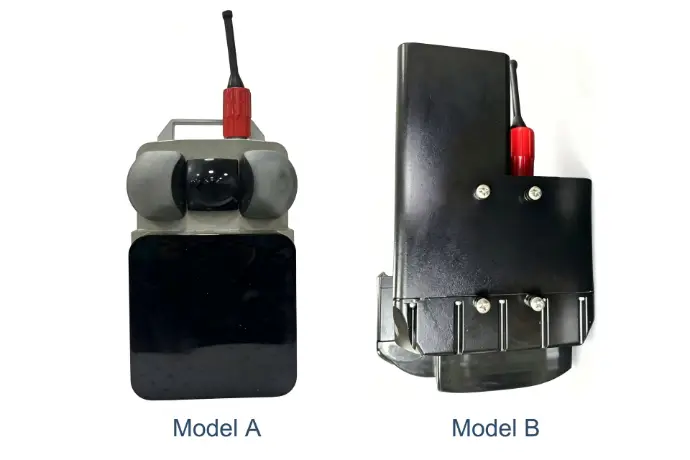
The 3D-300K is a true staring array: 576 receive elements in a 24 by 24 grid at 5 mm spacing, 30 kHz of bandwidth, forming beams in both angles at once. Physical size is 300 × 200 × 180 mm and 2.5 kg underwater, with 80 W of consumption and more than 48 hours of continuous operation.
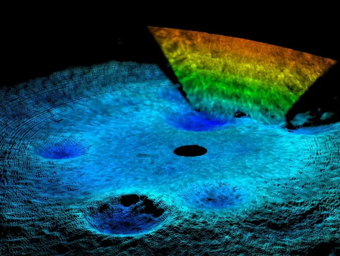
Its field of view comes in two versions, 50° × 50° and 55° × 55°. At 150 m the 50° fan covers roughly 140 m by 140 m of seabed, near 20,000 square metres, in a single look. That coverage per ping is what a mechanical scanner cannot match: the same area scanned line by line at 0.1° would take minutes.
The honest limit is the update rate. A ping to 150 m and back takes 0.2 s, so the maximum possible refresh at full range is 5 Hz, and the quoted 2–20 Hz range is range-dependent — 20 Hz needs the target inside 37.5 m. At 150 m you get about 5 volumes per second, a 50 by 50 angular grid sampled every 3 cm out to 150 m is on the order of twelve million voxels per frame, which is why every practical system decimates before display.
Mechanical scanning: 360° coverage and millimetre points
The MiniUAC-4001 solves the coverage problem differently. A single-beam head sweeps 360° horizontally and 216° vertically, which is the entire water column around the instrument, and 512 beams are synthesised along the sweep. Frequencies are 750 kHz and 1 MHz on the A0710 version, 1.2 MHz on the A1200, with 50 m and 40 m of range respectively.
Two numbers deserve attention. Angular resolution reaches 0.1°, which at 5 m is under a centimetre, and range resolution is quoted as "range-dependent, minimum 1 mm" — that word "minimum" is doing real work, because at 50 m the achievable range resolution is coarser than at 2 m. Blind zone is under 0.2 m, which matters when the instrument is mounted on a manipulator arm and the target is close.
The second number is time. At 0.1° the full circle needs 3600 lines, and at the maximum 100 lines per second a complete panorama takes about 36 seconds. That is a fine cadence for a static inspection — a bridge pier, a turbine foundation, a wreck — and a poor one for a moving vehicle. For motion the scanner offers a sector scan mode, trading coverage for refresh, which is exactly the right trade and worth specifying explicitly.
Power is the other surprise: about 5 W average with peaks under 10 W, in a 110 mm housing weighing 1.8 kg in air. A scanner that costs five watts can stay on for an entire dive, which is why it ends up on vehicles that cannot spare 80 W for an array.
Forward-looking multibeam: the middle ground
Between the two sits the forward-looking multibeam, which trades elevation for range and refresh. The MiniUAC-7512D is under 1 kg, 105 × 150 mm with a 72 mm diameter head, and offers 150° of horizontal field with 512 interpolated beams. At 750 kHz it reaches 120 m with 1° beams and 4 mm range resolution; at 1.2 MHz it reaches 40 m with 0.6° beams and 2.5 mm resolution, and a 40 Hz refresh that makes it usable as an obstacle-avoidance channel on a fast vehicle.
The UAC-FLS100 occupies the long-range end: 100 kHz, 0.96° angular resolution, 105° × 26° imaging fan that narrows to 7° in collision-avoidance mode, and a detection range of 500 m or more for a −15 dB target in good water. At 22 W typical and 30 kg in titanium, it is an instrument for a work-class vehicle rather than a small one.
The narrowing vertical fan in avoidance mode is not a gimmick. A 26° fan at 500 m covers a vertical slice 230 m tall, most of it water or seabed far above the vehicle's path; a 7° fan covers 61 m, which is the slice that can actually collide with you. Fewer beams wasted means more pings per second on the part of the scene that matters.
Update rate, data rate and what the platform can absorb
Every 3D sonar is limited by the same round-trip arithmetic as a side-scan: no refresh faster than c/2R. That single line explains most of the quoted ranges:
| Range | Round trip | Max refresh |
|---|---|---|
| 10 m | 13 ms | 75 Hz |
| 37.5 m | 50 ms | 20 Hz |
| 150 m | 200 ms | 5 Hz |
| 500 m | 667 ms | 1.5 Hz |
Then comes the data question. A 512-beam scanner producing 100 lines per second generates about 51,000 points per second before decimation; a staring array refreshing five times a second produces a frame of millions of voxels before decimation. Either is comfortable on Ethernet and awkward on a serial link, and either will fill a small vehicle's storage in an hour of continuous operation. Plan the logging policy before the survey, not after.
Choosing between the three geometries
The decision is a triangle between coverage, detail and refresh, and a project can hold two of the three.
Static inspection, centimetre detail, full water column. A mechanical scanner. 0.1° and 1 mm at short range, 360° × 216° coverage, five watts. Accept 36 seconds per panorama and use sector scan when the target moves.
Moving platform, volumetric awareness, no mechanical wear. A staring array. 50° × 50° at 150 m in one look, 5 Hz at full range, no rotating parts to fail. Accept metre-scale voxels at long range.
Obstacle avoidance and pilotage at speed. A forward-looking multibeam. 150° horizontal, 40 Hz refresh, 1 kg. Accept that elevation is compressed and that "3D" here means a 2.5D image.
Two failure modes recur. The first is buying a scanner for a moving vehicle and discovering the panorama cadence; the second is buying an array for close inspection and discovering the voxel width. Both are visible in the arithmetic above before any purchase order is written. Geometry questions that are not covered here — including how imaging sonars compare with multibeam echosounders for depth — are discussed in the imaging sonar forum thread.
FAQ
Is 3 cm range resolution the same as 3 cm image resolution?
No. Range resolution is the voxel thickness along the acoustic axis and comes from bandwidth. Image resolution across the fan comes from angular resolution multiplied by range, so a 1° beam is 2.62 m wide at 150 m. Both numbers appear on the same datasheet and describe perpendicular axes.
Why is the quoted update rate a range?
Because the sound has to travel out and back. At 150 m the round trip is 0.2 s, which caps refresh at 5 Hz regardless of processing power. Shorter ranges allow faster refresh, which is why the specification reads as a range rather than a single figure.
Can a mechanical scanner be used on an AUV?
Yes, if the mission accepts the cadence. A full panorama at 0.1° takes about 36 seconds; a sector scan over the sector of interest can run several times faster. The instrument is small and draws about 5 W, which suits vehicles with tight power budgets, but a fast transect is the wrong application.
What does an array give that a scanner does not?
Simultaneity. A staring array captures the whole fan in one ping, so a moving platform sees a coherent volume rather than a mosaic assembled over 36 seconds. The price is angular resolution: 1° against 0.1°.
Do I need a 3D sonar at all for obstacle avoidance?
Usually not. A forward-looking multibeam with a narrow vertical fan is cheaper, lighter and faster for that job, and the 2.5D image is sufficient because avoidance needs presence and bearing rather than shape. 3D becomes worthwhile when you need to measure a volume, not just detect an edge.


3D Imaging Sonar: Voxel Size, Coverage and Which Geometry