Side-scan sonar is sold on two numbers: how far it reaches sideways, and how small a thing it can show. Both are true and neither is independent, because swath and resolution trade against each other through frequency, and both are limited by geometry that the brochure does not draw. This note takes the UAC side-scan family as the worked example and shows where each number comes from, so a survey specification can be written from physics rather than from adjectives.
Two resolution numbers, and only one of them is about object size
A side-scan spec sheet usually prints resolution as a pair: 8.0 cm × 2.5 cm for our 300 kHz unit, 6.0 cm × 2.5 cm for the 450 kHz, and a single 1.5 cm for the 750 kHz. Those numbers describe two different axes.
The small figure is the range resolution: the ability to separate two targets at slightly different slant ranges, perpendicular to the track. It comes from the pulse bandwidth, not from the beam.
The large figure is the along-track pixel: how far the vessel advances between samples at rated range. It comes from the beam width and the ping rate, and it degrades linearly with range.
A 2.5 cm range resolution does not mean the sonar sees a 2.5 cm object at 250 m. It means that, once something is detected 250 m off the trackline, its distance from the trackline is known to about 2.5 cm. Whether it is detected at all, and how it appears along the track, is decided by the beam footprint and the pulse length.
Range resolution comes from bandwidth, not from frequency
The range resolution of any pulsed sonar is approximately half the pulse length in water:
dR = c / (2 B)With 1500 m/s sound speed, a 30 kHz bandwidth gives 2.5 cm, a 60 kHz bandwidth gives 1.25 cm, and a 25 kHz bandwidth gives 3 cm. That is why our 450 kHz unit publishes 2.5 cm from its 30 kHz band, the 750 kHz unit publishes 1.5 cm from its 60 kHz band, and the 300 kHz unit publishes 2.5 cm — a figure that implies roughly 30 kHz of effective bandwidth rather than the 25 kHz nominal, which is what a well-shaped CHIRP pulse can deliver.
The lesson is that resolution in range is bought with bandwidth, and bandwidth is available at any centre frequency. A 300 kHz system with a wide band is not automatically coarser than a 750 kHz one; what the higher centre frequency really buys is a narrower beam for the same aperture, and therefore a smaller along-track footprint and a smaller transducer.
The along-track footprint is the real limit
Along-track resolution is set by the horizontal beam width projected onto the seabed:
footprint = R × thetawith theta in radians. Our three units measure 0.22°, 0.2° and 0.25° horizontally, which is 3.8, 3.5 and 4.4 milliradians:
| Unit | Beam (horizontal) | Footprint at 50 m | At 100 m | At rated range |
|---|---|---|---|---|
| UAC-300S | 0.22° | 0.19 m | 0.38 m | 0.96 m at 250 m |
| UAC-450S | 0.2° | 0.17 m | 0.35 m | 0.70 m at 200 m |
| UAC-750S | 0.25° | 0.11 m | 0.22 m | 0.33 m at 75 m |
Read the last column carefully, because it is the number that decides whether a target is identifiable. At 250 m the 300 kHz beam is about a metre wide along the track. Two objects a metre apart on the same line of investigation merge into one return no matter how good the 2.5 cm range resolution is. Come in to 100 m altitude and the same system resolves 0.38 m; come in to 50 m and it resolves 0.19 m.
This is also why a survey plan is written as an altitude, not as a swath. The swath is a consequence of the altitude and the vertical fan, not a free parameter.
Swath, altitude and the geometry that keeps the seabed in view
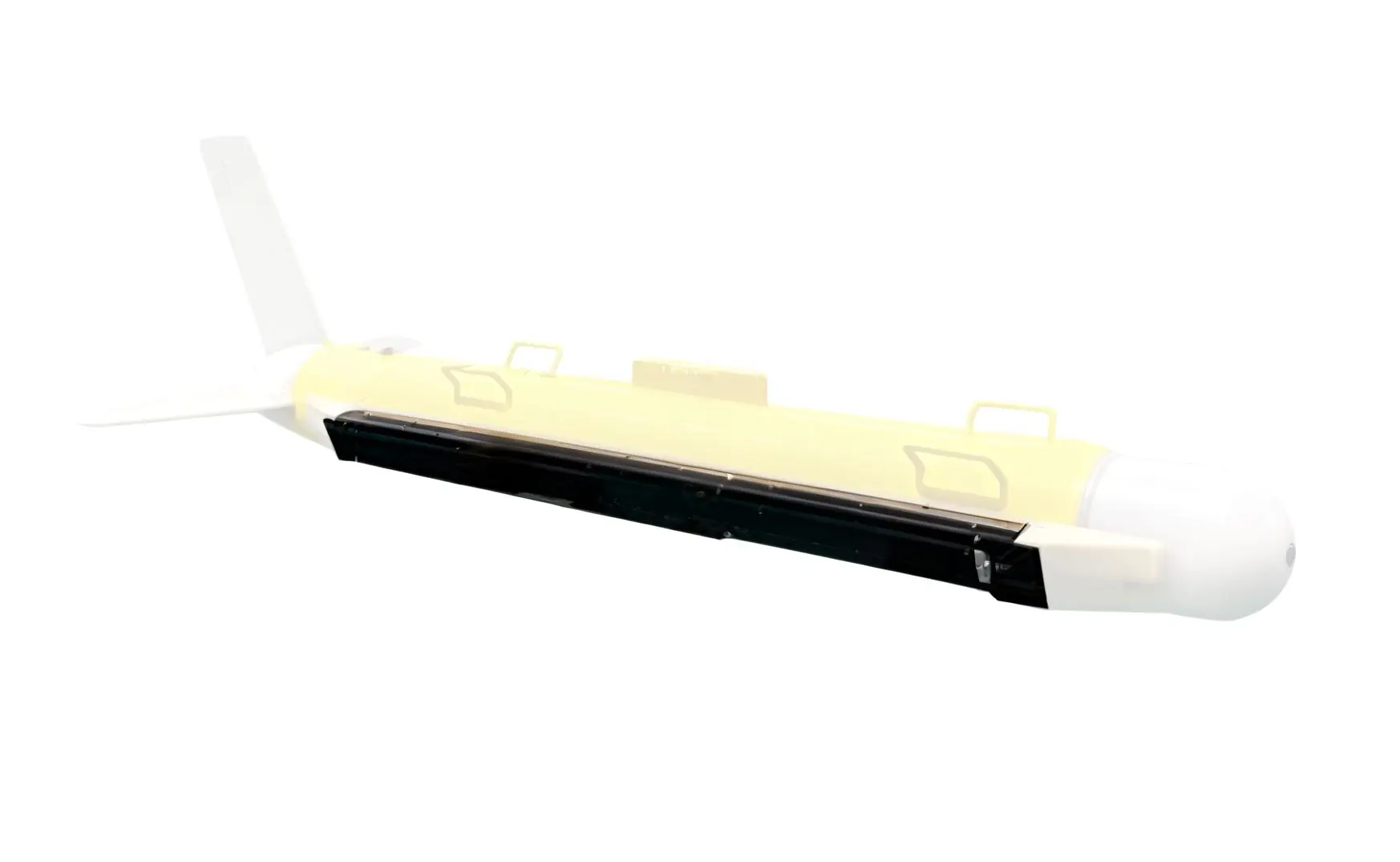
A side-scan transducer radiates a thin horizontal fan and a wide vertical one. Our units use 40°, 36° and 36° vertical, so the fan spans a band of grazing angles rather than a single line.
If the fan is mounted at the usual 30° depression, a 40° vertical opening covers 10° to 50° depression. At 50 m altitude that puts the near edge of the coverage at 50/sin(50°) ≈ 65 m from the trackline, and the far edge at 50/sin(10°) ≈ 288 m. The rated 250 m swath is the far edge, and it is only reachable when the altitude is high enough and the seabed is not rising faster than the fan.
Two practical consequences follow. Flying low narrows the swath but sharpens the pixels; flying high widens the swath and blurs the along-track axis. And in shallow, sloping or heavily dredged areas the far edge of the fan may be looking at the water column rather than the seabed, which is why experienced operators plan overlapping lines rather than maximum-swath lines.
Speed and ping rate: why a wide swath needs more than one beam
A sonar cannot ping faster than the sound can travel out and back:
ping rate <= c / (2 R)At 250 m the round trip takes 0.33 s, so the maximum is 3 Hz. At 10 knots the vessel advances 5.14 m/s, which is 1.71 m between pings against a 0.96 m footprint — a 44 percent gap along the track. Single-beam side-scan at 250 m swath and 10 knots cannot cover the seabed, and no amount of post-processing invents the missing returns.
There are exactly two honest fixes. Slow down: 0.96 m at 3 Hz is 2.88 m/s, about 5.6 knots, which is the speed at which a gapless 250 m swath becomes possible. Or use several beams across the track, which is what the 1–20 beam adaptive setting on our 300S and 450S does — more beams per ping at higher speed, fewer at lower speed, keeping the along-track sampling interval below the footprint.
At the other end of the family the constraint disappears. The 750 kHz unit pings at up to 10 Hz over 75 m, and at 5 knots it advances 0.257 m between pings against a 0.33 m footprint. High frequency is a poor choice for swath and an excellent choice for speed, and the numbers say so without any marketing.
| Parameter | UAC-300S | UAC-450S | UAC-750S |
|---|---|---|---|
| Centre frequency / bandwidth | 300 kHz / 25 kHz | 450 kHz / 30 kHz | 750 kHz / 60 kHz |
| Swath per side | 250 m | 200 m | 75 m |
| Range resolution | 2.5 cm | 2.5 cm | 1.5 cm |
| Max survey speed | 10 kn | 8 kn | 5 kn |
| Depth rating | 300 m | 600 m | 500 m |
| Power | 35 W typical | 33 W typical | 10 W typical |
| Transducer mass | 6.5 kg per side | 2.1 kg per side | 0.5 kg |
Integrated packages for USV and ROV work
The three-frequency line assumes a vessel with a deck, a winch and a separate electronics pod. Small platforms do not have those luxuries, and the answer is integration.
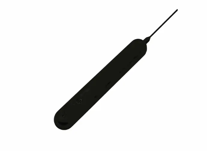
The MiniUAC-2003 puts side-scan, down-scan and a depth sounder in a single 377 × 57 × 31 mm housing that needs only power and Ethernet, drawing 5 W average with peaks under 20 W. Two versions are offered: 450 kHz with a 0.6° horizontal beam and 150 m per side, and 900 kHz with 0.3° and 75 m per side. Their published trackline resolutions, 0.21 m at 20 m altitude for the 450 kHz version and 0.11 m for the 900 kHz, are exactly R × theta — 0.21 m and 0.105 m — which is a useful reminder that the vendor's own figures obey the same geometry as everyone else's.
Weight matters as much as power on a small vehicle: 900 g in air and 300 g in water for the 300 m aluminium version, 1.5 kg and 900 g for the 1.5 km titanium version. On a 6 kg ROV payload that is the difference between one sonar and two.
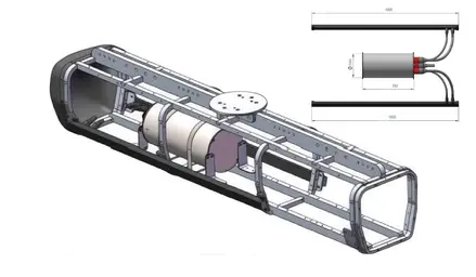
For platforms that want a wider acoustic toolkit in one package, the compact side-scan series includes the TFSS-4510, a triple-frequency all-in-one that combines side-scan with a bottom-scan channel. The trade is the familiar one: more channels and more coverage in the same housing, against a housing that is no longer free to place anywhere.
Specifying a side-scan sonar for a survey
Four questions, answered in this order, will produce a specification that matches the site.
What is the smallest object you must detect, and at what range? Object size sets frequency and altitude. A 0.3 m target at 250 m needs a beam of about 0.07°, which no 300 kHz side-scan reaches; it needs a shorter range or a higher frequency.
What altitude can you fly? Altitude sets swath through the vertical fan, and sets footprint through the horizontal beam. A 200 m swath at 30 m altitude is not achievable with a 36–40° fan; the geometry will not close.
What speed does the survey plan allow? Speed and ping rate decide whether the along-track sampling is gapless. If the answer is "10 knots at maximum swath", the honest answer is a multi-beam configuration or a narrower swath.
Where does the data go, and in what format? Ours record to DAT or standard XTF, with an SDK for secondary development. XTF matters if the deliverables feed a third-party mosaic package; a proprietary format matters if the deliverable is a report rather than a dataset.
One warning worth stating plainly: a side-scan image is a geometric projection, not a photograph. Shadows run away from the trackline, heights are inferred from shadow length, and a target in the near field is compressed by the grazing angle. Any interpretation workflow that treats the image as a plan view will misplace objects by metres at long range.
FAQ
Is a higher frequency always better for resolution?
For along-track resolution, mostly yes, because the same aperture gives a narrower beam at a higher frequency. For range resolution, no: that comes from bandwidth, and a 450 kHz system with 30 kHz of bandwidth resolves 2.5 cm just as a 750 kHz system with 30 kHz would. What you pay for the higher frequency is swath and power, not resolution in range.
Why does my 250 m swath look narrower than the specification?
Because swath is measured at a rated altitude and a flat seabed. Fly lower, or survey a slope, and the far edge of the fan leaves the seabed. The rated figure also assumes the maximum detection range, not a guaranteed detection at that range for a small target.
Can side-scan replace a multibeam echosounder for bathymetry?
No. A side-scan measures acoustic amplitude along a fan and infers shape from shadows; it does not measure depth per beam. For depth you need either a multibeam echosounder or a side-scan with an interferometric option, and the choice between imaging and sounding is discussed in the imaging sonar forum thread. Side-scan remains the better tool for texture, target detection and debris.
What does CHIRP change?
CHIRP sweeps the transmit band instead of emitting a single tone, which raises the effective bandwidth for a given peak power and improves both range resolution and signal-to-noise at long range. It does not change the beam width, so the along-track limit stays exactly where the geometry puts it.

Side-Scan Sonar: Swath, Resolution and Frequency Choice